+Introduction

In computer science, 'recursion' refers to a strategy where the solution to a problem can be solved using solutions to smaller versions of the same problem. In computer programming, such systems are defined using 'recursive functions' which are basically functions that can call themselves. These kinds of functions are impossible to define in Grasshopper because there is no way to feed data from a function back into itself. Using Python, however, we can easily create such functions by having the function define its output based on the outputs of modified versions of itself.

These recursive calls to the same function create a kind of spiral behavior defined by subsequent executions of different versions of the same function. By default this recursive behavior will create an infinite spiral, similar to the infinite while Loop we saw in a previous guide. If you don't provide any way for the recursion to stop, the function will keep calling itself for eternity, which will simply cause your script to crash. We can prevent this by defining a Conditional inside the function that specifies a 'termination' or 'exit' criteria which stops the function from calling itself. Once the final function call has terminated, its return is fed all the way back through all the function calls until the final solution is returned.

The concept of recursion is incredibly powerful, and there are many useful applications for recursion in computer programming. At the same time, the nested behavior of recursive functions can be difficult for people to understand intuitively, which is why recursion tends to be a difficult subject for people just starting out in programming. To start to gain an intuition for how recursive functions work, let's create a simple example of a recursive function that can add a sequence of numbers up to a certain value. We won't be using any geometry yet, but you can try this code directly in a Python component in Grasshopper.

def addRecursively(value):
    if value == 0:
        return value
    return value + addRecursively(value-1)
print addRecursively(3)
# prints 6

If you run this script you should see 6 as the result in the output window, which is indeed the result of summing 1 + 2 + 3. You can see that addRecursively() is a recursive function because it calls itself within its definition. To see how this function works, let's step through all of the function calls that lead to the final solution.

The first time we call the function we pass in the number three, which is brought into the function in the variable 'value'. The function first checks if this value is equal to 0, and if it is it simply returns the value. This causes the function to return 0 if its input is 0, which is a valid solution to our summation problem. This Conditional is the 'termination criteria' of our function. In order for our function to not enter an endless spiral and crash, we have to ensure that this criteria is met at some point. In our case we must ensure that the value input into the function eventually becomes 0.

In our case the value is '3' so the Conditional is skipped, and the function instead returns the input value added to the results of the same function with an input of one minus the value. This causes the function to execute again, this time with an input of '2'. The original function will now wait until it gets the return from this new function, at which point it will return the value of the new function plus 3.

To get a better understanding of how this works, let's visualize the sequence of calls and returns:

addRecursively(3) --> 3 + _
    addRecursively(2) --> 2 + _
        addRecursively(1) --> 1 + _
            addRecursively(0) --> 0
            1 + 0 --> 1
        2 + 1 --> 3
    3 + 3 --> 6

You can see how this forms a nested set of calls to the same function, with each function waiting for it's child function to return its value before generating its own return.

What if we want to add an arbitrary list of numbers instead of a sequence of numbers? To do this we can create a variation of our addRecursively() function which takes in a list of numbers and operates on them one by one:

def addRecursively(values):
    if len(values) <= 0:
        return 0
    value = values.pop(0)
    return value + addRecursively(values)
print addRecursively([1,3,5])
# prints 9

In this case the input into the addRecursively() function is a list of values. The termination criteria is when there are no more items in the list, at which point the function returns 0. If there is at least one item remaining in the list, the function uses the list's .pop(i) method to remove the first element from the list and store it in the 'value' variable. Then the function returns this value added to the return of the same function called with the new version of the list which has the first value removed. We can visualize this behavior in the same way as before:

addRecursively([1,3,5]) --> 1 + _
    addRecursively([3,5]) --> 3 +
        addRecursively([5]) --> 5 + _
            addRecursively([]) --> 0
            5 + 0 --> 5
        3 + 5 --> 8
    1 + 8 --> 9

We can use this list-based method of recursion to parameterize the behavior of any recursive function with a list of parameters. In the addition case, the numbers in the list can be thought of as parameters that control the behavior of the addition over time. In the same way, we can imagine a set of parameters which control the behavior of any recursive function that is executed the same number of times as there are parameters.

+Exercise: Branching tree

In this exercise, we will write a recursive algorithm that generates a branching tree structure based on a sequence of parameters which we can modify to control the shape of the tree.

Branching systems and other fractal geometries commonly found in nature are often modelled using recursive functions because they are self-similar, meaning that the same behavior is exhibited at various scales throughout the structure. For example, the branching of a set of large branches from the trunk of a tree is similar to the branching of a smaller set of branches from each of these branches.

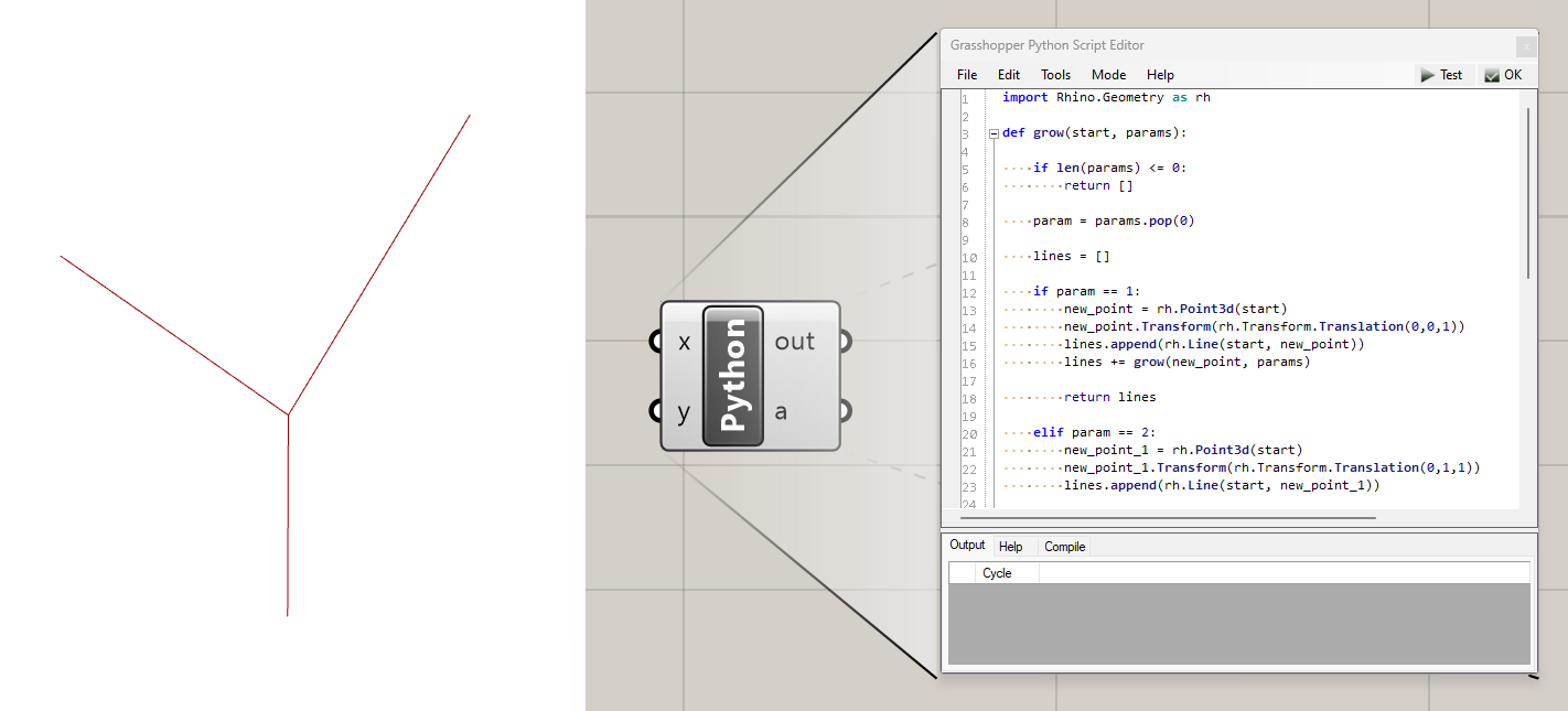
Here is the code for a basic branching algorithm in Python. You can paste it directly into a new Python component in Grasshopper.

import Rhino.Geometry as rh

def grow(start, params):

    if len(params) <= 0:
        return []

    param = params.pop(0)

    lines = []

    if param == 1:
        new_point = rh.Point3d(start)
        new_point.Transform(rh.Transform.Translation(0,0,1))
        lines.append(rh.Line(start, new_point))
        lines += grow(new_point, params)

        return lines

    elif param == 2:
        new_point_1 = rh.Point3d(start)
        new_point_1.Transform(rh.Transform.Translation(0,1,1))
        lines.append(rh.Line(start, new_point_1))

        new_point_2 = rh.Point3d(start)
        new_point_2.Transform(rh.Transform.Translation(0,-1,1))
        lines.append(rh.Line(start, new_point_2))

        lines += grow(new_point_1, params) + grow(new_point_2, params)

        return lines

    else:
        return lines

params = [1,2,0]
a = grow(rh.Point3d(0,0,0), params)

This code sequentially generates a branching structure based on a set of parameters which can be 0, 1, or 2. The grow() function takes in a starting point and creates zero, one, or two new branches based on the first parameter in a set. It then calls the grow() function again with the end of each new branch as the starting point and the reduced parameter list. The output of the grow function is a list of lines representing the branches. Let's step through the function calls using an example set of parameters [1,2,0] to see how it works.

The first time we call the grow function we pass in a new point at the origin [0,0,0] along with the full set of parameters. At this point, the length of the parameter list is 3, so the termination criteria is not met and the function continues. Next the function pops the first parameter from the list and stores it in the param variable. It also creates an empty list called 'lines' to store the geometry of the branches it creates.

Now the function encounters a set of Conditionals which do different things depending on the value of the current parameter. If the parameter value is '1' it makes one new branch by creating a new point as a copy of the start point:

new_point = rh.Point3d(start)

It then moves that point one unit in the z direction to create a vertical branch:

new_point.Transform(rh.Transform.Translation(0,0,1))

It then creates a new line between the start and new point and appends it to the lines list:

lines.append(rh.Line(start, new_point))

Finally, the grow() function is called again using the new end point as the start point of the new branch and the reduced set of parameters (with the first parameter removed by the previous pop() operation). The results of this function call are added to the list of lines which are then returned from the original call to the grow() function.

The behavior for a parameter value of '2' is similar except we now create two diagonal branches instead of one vertical one and call the grow() function twice before returning the lines list. At first it might seem that calling the function twice in one line would pass the same parameter values to both new branches, so that we would end up with more branches that starting parameter values. In fact, when we use variable names in Python we are actually using references to the variable stored somewhere in memory, which means that all the function calls are actually interacting with the same exact list. This means that when one function pops a value out of the list, the list is affected for all subsequent functions, even if they are called later on the same line.

In this example the first call to the grow() function pops one of the parameters from the list so it is already reduced when the second grow() function is executed later in the line. In this case this is what we want since we only want each parameter to be considered once. If we actually wanted to pass the same exact parameter list to both function calls we would first have to make a copy of the list. To make sure each parameter is only being used once we can print the values in the parameter list at the beginning of each function call:

The final Conditional in the function is an else statement that captures any other possible parameter value and results in the return of an empty list. This includes the parameter 0 which we expect to terminate the branching procedure. Although we could have programmed the behavior for our expected inputs of 0, 1, and 2 through their own explicit Conditionals, it is good practice to nest all of the conditions together using elif statements and have a final else condition at the end to capture all other cases. This provides a fail-safe termination condition that ensures that the recursive function will always terminate even if you enter an unexpected value by accident.

For our parameter set of [1,2,0], the first call to grow() generates one vertical branch and calls grow() again. The second call creates two diagonal branches and calls grow() two more times. The first of these calls returns an empty list because the parameter is '0'. The second call also returns an empty list because there are no more parameters in the list. This results in the structure seen above. Here are some other possible structures based on different sets of input parameters. Note that the '0' parameter has the effect of stopping any branching path, so any sequence starting with '0' will produce no branches since the behavior is stopped at the first step.

This example shows the power of recursive functions in defining complex forms based on a small set of abstract parameters. However, the use of recursion is not restricted only to branching problems. In fact any system can be implemented using recursive functions as long as it can be described based on smaller versions of itself. In a later exercise, we will see how a similar kind of recursive algorithm can be used to subdivide a given space into several other spaces.

+CHALLENGE 8: Branching tree

Download the starting Grasshopper file and open it up in a blank Rhino and Grasshopper file. The model's Python component contains the definition of the tree model developed in class. It also includes a list of input parameters that are passed into the Python component from a Panel component, and uses a Pipe component to visualize the branch geometry as closed cylinders.

Your task is to add additional code within the Python script to define a new branching behavior for the '3' parameter that creates the branching seen in the screenshot below. You should only add code within the elif param == 3: code block starting on line 35 of the Python script. You should not need to modify anything else about the code, the Grasshopper definition, or the set of parameters.

HINT: Currently, the behavior for the parameter '3' is the same as for '0' or any other undefined parameter. It simply returns the empty list, stopping the branching at the current point. To get the branching result shown, you should add a logic similar to the one for the parameter '2', but generating two branches going in the 'x' instead of the 'y' direction.

+Conclusion

In this exercise, we created a recursive function that can generate a branching tree based on a set of parameters.