
colidescope
/guides/ 01-intro-to-grasshopper-01-getting-started
colidescope
/guides/ 01-intro-to-grasshopper-01-getting-startedIntro to Grasshopper
The first step on your Grasshopper journey, this guide covers the basics of the tool and demonstrates it with a small exercise
Getting started with Grasshopper
In this section you will get your first introduction to the Grasshopper visual scripting environment
¶Other sections in this guide
| Intro to Grasshopper | |
|---|---|
| 1 | Getting started with Grasshopper |
| 2 | Exercise: Hello Grasshopper |
¶What is Grasshopper?
Like any programming environment, Grasshopper allows you to create algorithms, or sets of instructions, for telling a computer what to do. In traditional programming, these instructions are written using programming languages, text-based systems that follow strict formatting rules and have specific vocabularies for describing computer operations. With visual programming, the instructions are described in a visual interface using a set of nodes, or components, that describe operations, and a set of lines, or wires, that create connections between them. The layout of these components and wires is stored in a visual script or definition that can be visualized and edited in the Grasshopper canvas.
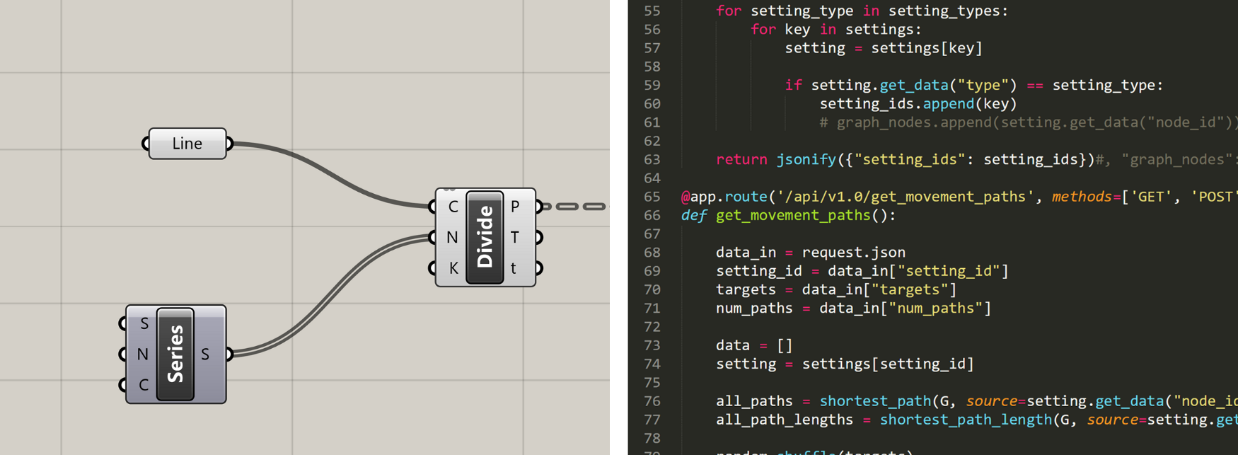
Visual programming (left) and text-based programming (right)
In mathematical terms, you can think of the components as functions which take in inputs and generate outputs. The wires then are the way in which data is passed between the inputs and outputs of different functions. Although text-based and visual programming can accomplish many of the same things, a visual interface can be easier to learn and more intuitive to use for designers, who tend to be more visually oriented and don't typically have a background in coding.
¶How does Grasshopper connect to Rhino?
Like most computer software, Rhino has two components — the front-end graphical user interface (UI) with which users interact, and a backend system that contains all the logic for what the program can do. In a CAD program like Rhino, the front-end contains the visual display of the geometry and a command-input system that allows users to run commands to generate geometry while providing inputs and getting visual feedback from the display. On the backend, there is a code library that defines the functionality behind all of the geometric commands, along with other functionality needed by Rhino such as saving and loading files.
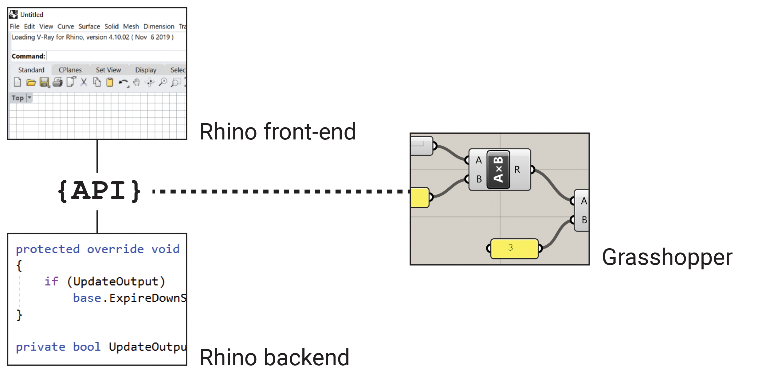
Like many modern software, Rhino exposes its backend system through an Application Programming Interface (API), which allows third-party developers to build functionality on top of Rhino’s backend system while bypassing the front-end user interface. Grasshopper utilizes this API to expose the geometric operations as individual components, allowing users to craft their own automated workflows using Rhino’s backend. The Rhino API and how it is used by both Grasshopper and Python to access Rhino's functionalities will be discussed in detail in a later guide.
¶Getting started in Grasshopper
Grasshopper started its life as a plugin for Rhino which you had to download and install separately. Since version 6, Rhino now has Grasshopper built-in, so if you are using Rhino 6 or later, you don’t need to install any additional software to use Grasshopper. You can start Grasshopper either by clicking the Grasshopper button in the toolbar or by typing Grasshopper in the Command line.
When you start Grasshopper, it will open up in a new window on top of your Rhino interface. The Grasshopper interface consists of two main parts: the components library at the top, and the canvas below.
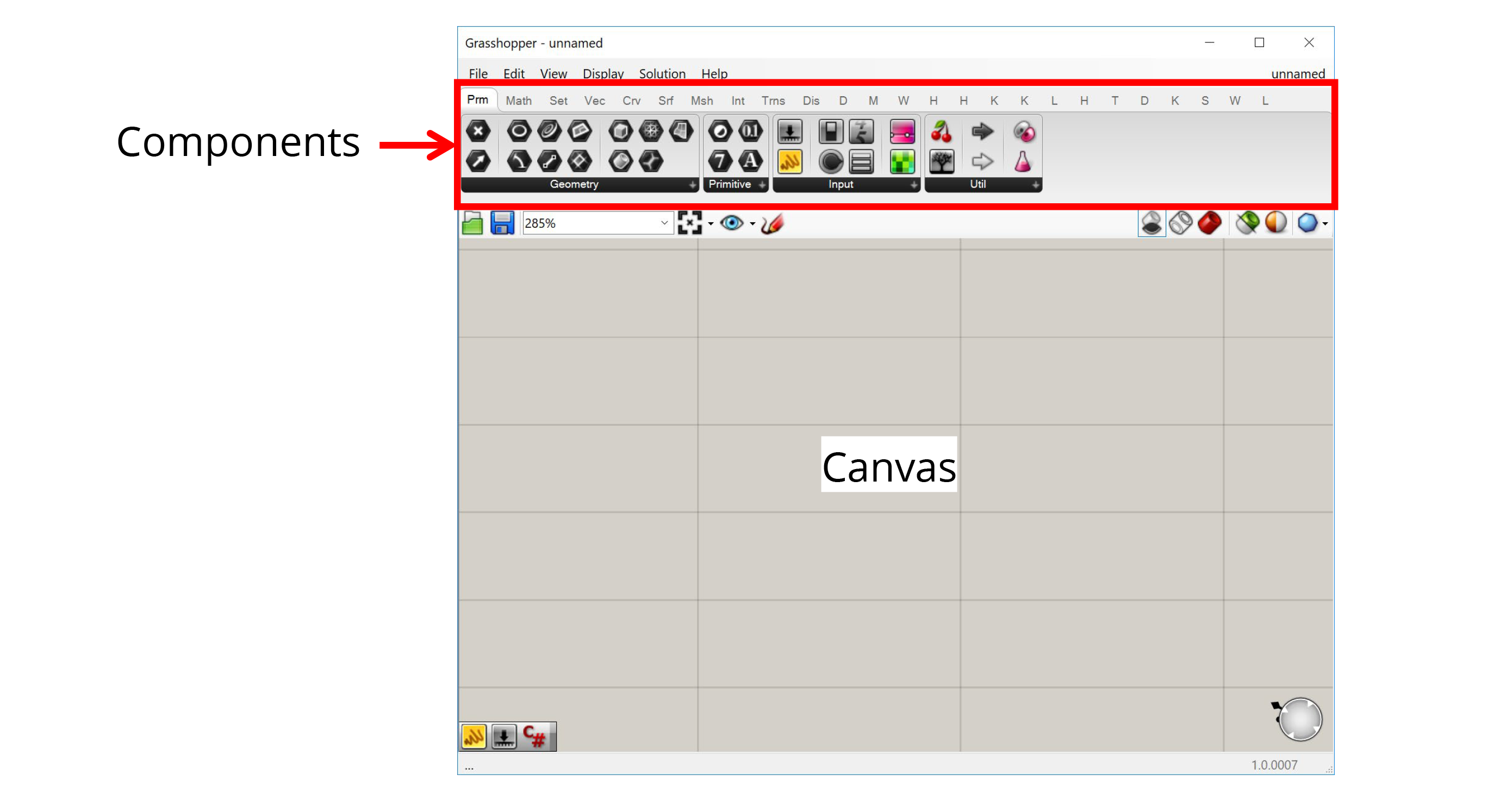
¶The components
The components library contains all the components that are available to use in your model. Grasshopper comes pre-loaded with a large number of basic components, and you can also download libraries of custom components made by other users (more on loading libraries later). Each component is represented by an icon in the toolbar, and they are organized according to their function or the library they come from.
¶The canvas
The canvas is the most important part of Grasshopper. It is the visual environment in which you develop your Grasshopper models. To create a model, you drag components from the top toolbar onto the canvas, and then connect them together with wires by clicking and dragging between an input and output node.
You can think of the Grasshopper window as a separate "view" into your Rhino file. The Grasshopper model developed within the canvas has a connection to the Rhino model from which it was launched, so you should think of both Rhino and Grasshopper working together in a common environment, using their own separate interfaces.
When you develop geometry in Grasshopper, you will see this geometry visualized within the Rhino viewport. You can also reference objects from Rhino into your Grasshopper definition. With certain objects like points, you even get an interactive widget that allows you to move the Grasshopper geometry directly within Rhino.
Any geometry developed within Grasshopper is considered "dynamic geometry" because it does not actually exist in the Rhino model, but is only displayed for preview purposes in the viewport. Because of Grasshopper's connection to the Rhino model, however, you can take any geometry developed in Grasshopper and "bake" it so it becomes a permanent part of the Rhino file.
Because Grasshopper has its own interface and stores its own data, the definitions you develop in Grasshopper need to be saved to a separate file which usually has the extension .gh or .ghx. This file is separate from the .3dm file which contains your Rhino model data. This means that when you are working with Grasshopper, you typically are working in two separate files: a Rhino document and a Grasshopper model that is connected to it.
¶The Grasshopper community
One of the best features of Grasshopper, and one of the key factors behind its success, is the amazing community of designers and programmers that’s grown around it.
Designing computationally can be a very challenging and creative process. When you are building something totally new there are not always standard answers out there for how to solve the problems you might run into. In such cases it is useful to have a strong community of fellow users who can share experiences and help each other to overcome challenges in a collaborative way.
Because of its connection with computer programming, computational design inherits a lot of the community and open-source culture of the software development industry. A great way to engage with the Grasshopper community is by visiting the Grasshopper forum: https://discourse.mcneel.com/c/grasshopper-developer.
At this point, Grasshopper is old enough and the community of users is large enough that you can usually Google Grasshopper + whatever your issue is and get results from the Grasshopper forum (or occasionally private blogs or video tutorials) discussing the same issue.
¶Exercise: Hello Grasshopper!
Learning new software can be a difficult and laborious process, especially with a more technical and analytical tool such as Grasshopper. The best way to stay motivated is to devote enough time during your training process to actually working with the tools and learning their capabilities first hand. For this first exercise, let’s start with something simple that nevertheless shows some of the key concepts behind Grasshopper. We will create a 5-component definition that generates a series of circles based on one number slider.

¶Step 1: Define the base point.
We need somewhere to start with our definition. A good place to start is defining a location where our circle geometry will be generated. We can do this using a point object, which defines a location in space based on its x, y, and z coordinates.

To define a point in Grasshopper we can use the Point component. This defines a point in Grasshopper by referencing a point already in the Rhino model or by creating one directly in Rhino. To place the point on the canvas, click the component in the toolbar, and while holding down the mouse button drag it onto the canvas. Release the mouse button to place the component on the canvas.

When you first place the component on the canvas it will be colored orange, which tells you that there is some kind of warning being generated by the component. In this case, it’s because we haven’t yet defined a point for the component, so let’s fix that in the next step.
Right-click on the Point component and select ‘Set One Point’. This will switch you over to the Rhino interface and ask you to select a location for the Point. Look at the command line and make sure the option for selecting the location is set to ‘Coordinate’. This will allow you to pick the location dynamically by clicking in the Rhino viewport. You can also type “0” and hit Enter to place the point at the model’s origin.
Once you place the point, you will be taken back to the Grasshopper canvas, where the component has now turned the default light grey color. You will also see a red cross in the Rhino viewport representing the location of the point defined in Grasshopper. Remember that this is just a visualization of the point, which only exists in Grasshopper and does not exist in the actual Rhino model. If you click on the Point component you will see a widget displayed over the point in Rhino which allows you to change its position interactively.

¶Step 2: Create a circle
Now that we have a point to work from, let’s use it to create a circle. To make sure you see the circle geometry properly, switch to either the Top or a 3d viewport in Grasshopper, centered on the point we just created.

To create a circle, we need to find the right component in the toolbar. Grasshopper actually has several different components for creating circles, which can be found in the ‘Primitive’ section of the ‘Curve’ tab five over from the left. The one you choose depends on how you want the circle to be generated. In our case, we will use the Circle CNR component, which generates a circle based on its Center-point, Normal vector, and Radius (CNR).
Drag a Circle CNR component out to your canvas and place it to the right of the Point component. As before, the component is orange because we have not supplied it with the data it needs to generate its output. To make the component work we need to supply this data through its input ports.
Let’s start by defining the circle’s center point by connecting the output port of the Point component to the ‘C’ input port of the Circle CNR component. When these components are connected, the point geometry stored in the Point component ‘flows’ to the Circle CNR component, where it is used to specify the center point of the circle created. It is important to understand that the geometry does not physically move between the components. The point geometry is still stored in the Point component, but is referenced by the Circle CNR component when it performs its task.

Once we define the circle’s center point, the Circle CNR component turns grey and you should see a red circle appear around your point in the Rhino viewport. The component is able to run and generate the circle geometry even though we did not supply the second and third inputs. This is because it has default values for those inputs stored within the component.

You can see these default values by hovering over the labels of the inputs. In this case, the component is using a unit Z vector as the default normal vector, and ‘1’ as the radius. We will discuss vectors in more detail in a later lesson so we won’t worry about it for now and leave the default Normal vector as it is.

To control the size of our circle interactively, let’s connect the Circle CNR component’s ‘R’ input to a Number Slider. You can find the Number Slider in the ‘Input’ section of the ‘Params’ tab, first from the left. Place a Number Slider component below the Point component on the canvas and connect it to the Circle CNR component’s ‘R’ input. You can now change the value of the Number Slider and see the circle changing size dynamically in the Rhino viewport. Since the range of the slider is set to 0–1 by default, you may have to zoom in on your viewport to see the circle.

¶Step 3: Divide the circle
Now that we have one circle, let’s make some more! To make more circles, we will need more center points to define their location. This time, instead of creating the points manually, let’s generate them from the geometry we’ve already created.

To generate a set of points, we can use the Divide Curve component. Like the related Rhino command, the Divide Curve component places a set of points at even increments along a curve to represent divisions within a curve. You can find this component in the ‘Analysis’ group in the ‘Curve’ tab fifth from the left. Place the component to the right of the Circle CNR component on your canvas, and connect the (C) output of the Circle CNR component to the (C) input of the Divide Curve component.

The Divide Curve component requires 3 inputs: the curve to divide (C), the number of divisions (N), and a True/False value for whether to split the curve at kinks before dividing. As before, the second and third inputs have default values, so as soon as you connect the circle to the curve input you should see a set of 10 points appear around the circle.
The Divide Curve component generates three different outputs, which you see represented by three ports on the component’s right side. The first output (P) stores the actual points, the second (T) stores the curve’s tangent vector at each point, and the third (t) stores the curve’s parameter values at each point.
¶Step 4: Create more circles
Now that we have some more points we can use them to define more circles using the Circle CNR component. If you want to reuse a component (or set of components) in your canvas you can easily copy and paste them using the ‘Ctrl+C’ and ‘Ctrl+V’ shortcuts. Copy and paste another version of the Circle CNR component and move it to the right of the Divide Curve component. You will see that the pasted copy keeps the same inputs as the original component, so in effect it is creating the same circle. To finish off our definition, let’s swap the new Circle CNR component’s (C) input to the new points stored in the Divide Curve component’s (P) output. This generates 10 more circles, one at each of the new points.

Notice that when we pass one point to the Circle CNR component we get one circle, and when we pass ten points we get ten circles. This is because the component runs once for each input supplied. We will discuss in more detail how Grasshopper handles multiple data streams, and how this affects how components run, later in the course.
¶CHALLENGE
Can you modify the definition to control the number of division points (and thus the number of circles generated) dynamically? Can you set it up so that the number of circles as well as their size is controlled through a single
Number Slider?HINT: since divisions happen in whole numbers you may have to change the range of the number slider to create values higher than 1.
¶Conclusion
In this exercise, we created a simple definition from five components that creates a set of related circles. Although it’s only a small example, it does illustrate the basic concepts of how we develop models in Grasshopper. Every Grasshopper model needs a starting point, and from there you build up complexity by passing data through more and more components.
As you get more experience with Grasshopper, you will see that learning the components is only the first step of becoming a great computational designer. The true skill of computational design is learning how to approach design problems computationally, and break down complex problems into a set of simpler problems that can be represented through the right set of components. You will get more practice with this as you work through the rest of the exercises in this guide.
That concludes this module, congrats! Now that you have a bit of hands-on experience in Grasshopper, you can go on to the next exercise, where we will dive deeper into the Grasshopper user interface.